Dynamic Function Market Makers

Dynamic Function Market Makers
Automated Market Makers (AMMs) have been extensively studied in DeFi and usually appear in the form of Constant Function Market Makers (CFMMs). I will discuss a more general class of AMMs called Dynamic Function Market Makers (DFMMs) for which CFMMs are a special case.
Key idea: CFMMs maintain a constant trading function while DFMMs can allow for the trading function to change.
What's the point?
Before I continue further, I don't want you to feel as if what you are about to read is abstract nonsense. The point of this model of DFMMs is to allow for more flexibility in the design of AMMs and to allow for more complex trading functions that can be tailored to an individual's desire. This particular design also allows for the tokenization of liquidity positions which can be used to create new financial instruments. None of what you are about to read is inherently unknown to the DeFi community, but I think that the DFMM framework presented here is a convenient formalism. Furthermore, making the mechanism design of AMMs rigorous allows for more principled analysis of their properties which in turn makes them easier to test and safer to operate.
With DFMMs, you get a derivative exposure on the tokens inside of the pool. The derivative comes in the form of a specially catered payoff curve or portfolio value function that can adjust over time and due to market state. However, you also get the benefit of being able to trade in and out of the position at any time and you do not need a counterparty. Furthermore, with tokenized LP positions, you can engage in borrowing and lending of liquidity positions which can be used to attain convex exposure. Last but not least, as now popular in DeFi, you can also use DFMMs to have a market-making-style derivative where you can also think about the location of your open two-sided orders (liquidity depth) at a given price.
With this in mind, we can consider the DFMM as a building block for decentralized portfolio management.
Background
There are many resources discussing CFMMs, but I recommend The Geometry of Constant Function Market Makers by Angeris et. al. In essence, a key result of the paper is that a CFMM's trading function is the boundary of a convex set of reachable states and there is a unique homogeneous trading function in an equivalence class of such functions.
Notation
We will use the following notation for a DFMM pool:
- is the trading function.
- are the reserves.
- are the pool parameters.
- is the liquidity which has dimensions of tokens.
- are the blockchain state. For instance, this could be block number and block timestamp or even functions applied to the previous state of the pool.
- is the pool state.
- is the share balance of a pool or user.
- is the share redemption rate.
- is the quoted price of the pool.
- is the fee parameter, i.e., a 30bps fee yields .
Note that I will later use for price so I apologize for the mix of notation but the context should be clear.
Rework
Let's rework the CFMM case just slightly to prepare for the DFMM case. In the referenced work, we have where the choice of image defines the boundary of a reachable set. Instead, consider where the second input is a liquidity parameter . To define the boundary of a reachable set, we pick and consider . That is, the set of reserves where (also called the kernel) where signifies an open input, i.e., .
Moving forward, we will consider the kernel of for which the CFMM is a special case where pool parameters are fixed, there is no influence from the blockchain state. Prices of tokens in the pool can still be defined as a map .
DFMMs
Picture a DFMM as a parameterization by of reachable sets in the set of all possible reachable sets . Naturally, the oracle-free parameter choices are those listed above as . For posterity, can be extended to be any parameter space that is appropriate for your application at hand and could include external data feeds such as market prices or volatility.
Scale invariance
We will work with an equivalent condition of being homogeneous (as described in Angeris et. al.) in reserves as we have found this be more computationally viable. Namely, consider functions for which the reserves such that defines a hypersurface in for which is solely a scaling factor. That is, if is a solution to
then if we scale by , we have that
for some so long as . This condition itself is weaker than homogeneity as we are not requiring that . In the case that , we say that is scale invariant in the reserves and we can see this is equivalent to homogeneity of degree in the reserves. To prove this, consider where . If is homogeneous, then
This must only be true if so by definition of we have the result.
Parameters
In a different scenario where the pool parameters and blockchain state changes: and , we can determine a new value of such that
This is to say that changing parameters while leaving reserves invariant may cause a change in liquidity parameter . We have examples of this in Dollar cost averaging, Covered call below, and Liquidity tracker strategy.
DFMMs as state machines
Allow us now to extend the state of the pool to include a share balance and a share redemption rate . Later on, this will let us tokenize liquidity positions. By abuse of notation, we will now think of
If you'd like, you can place and into as is a bit of a catch-all for any and all blockchain state.
Let be the current state of the DFMM at step (including our and as above), then the DFMM can be thought of as a state machine that takes in current and the next state and produces if and only if the pair is valid and the machine continues the state transition and otherwise produces (invalid) and rejects the state transition, halting progress. We use the machine's built in map where and .
The DFMM has two possible instructions each of which carry a payload of two states:
Definitions.
- () We say that a instruction is valid if and only if the new state is in the kernel of the extended trading function and if the fee yields at least . Concretely, assuming we can determine a-la Equation (1) and the tokens we tender are in the list , we get the expression:
- () We say that a instruction is valid if and if the LPTs are credited at the share redemption rate . If so, then the LP is credited LPTs upon allocation, and debited LPTs upon deallocation (hence and not ). Specifically:
For the definition, I should say that determining the from the parameter updates is not always possible analytically and may require a numerical solution such as bisection search.
For the , we are implicitly assuming pool parameter nor blockchain state values are changing within this instruction, though allowing for this is possible and would be a straightforward modification. Second, in the case the trading function is scale invariant, we get . Third, it follows that the quoted price is equivalent to the current quoted price . The fact that price is invariant under is under the assumption that only should lead to a change in quoted price from an AMM.
Let us illustrate these concepts with some examples.
Examples
We will provide two examples of CFMMs and their DFMM counterparts. First is the Geometric Mean Market Maker (GMMM) and the second is the Log Normal Market Maker (LNMM).
Geometric Mean Market Maker
The GMMM is a CFMM that maintains the following invariant:
where are the weights (i.e., is the portfolio weight of token ), and is the liquidity parameter which we can see has dimensions of tokens. In our notation before, and . We also require that and . Finally, the fee parameter is constant, and I dropped it from the notation of the pool state for this example.
This trading function is scale invariant. To see this, note
Remark. You could consider to be the trading function of the GMMM as the kernel is the same set and the kernel is all we need to definee when an instruction is valid. However, computationally it is better to work with as it is scale invariant in the reserves and liquidity parameter to be near 1 as opposed to . This matters for stability of numerical approximations.
Since this CFMM is scale invariant, if we change the reserves to via , then this is validated if .
As a DFMM
The DFMM counterpart allows for the weights be arbitrary functions of the additional parameters . We will denote the varying weights by where is a choice of blockchain state, i.e., we could let:
where is the block timestamp. Hence the state of our example DFMM is:
Dollar Cost Averaging
For simplicity, consider a pool with two tokens and with weights solely dependent on time. That is, we have and respectively. Then the DFMM trading function is:
where is the liquidity over time. As a reminder, since is dynamic and reserves may not change from one step to the next, will change over time along with based on our discussion in Parameters.
For sake of concreteness, we can let and take so that the weights are linearly interpolated between and . The pool will start out with weight on and weight on and end with weight on and weight on . This can be thought of as a means of dollar cost averaging from into over time .
Liquidity Update
Suppose that we want to update the liquidity of the pool at time to where . Then we can solve for such that . Quickly:
Visualization
Let's imagine now that we want to maintain the reserves and constant over time and we want to update the liquidity over time so that the reserves maintain on the graph of the trading function.
For instance, if we have and , then we can take , to be a point on the graph of the trading function.
Now, we can update to be for which we would find and if we updated again to , we would find .
See the figure below for a visualization of this process.
Volatility Targeting
Suppose that we want to maintain a constant volatility of the pool over time. Then we can define the volatility of the pool as the standard deviation of the price of the pool over time and if we know the volatilities of each token in the pool, we can pick a set of weights that will allow for the pool to attempt to maintain a constant volatility. This is certainly not a new idea as Aera provides this using Balancer and decentralized parameter submitters.
Log Normal Market Maker
The LNMM is a CFMM that maintains the following invariant:
where , is the inverse of the cumulative distribution function of the standard normal distribution, is the mean price of Token X with respect to Y, is the width parameter, is the time parameter, and is the fee parameter. Note that this is also scale invariant in the reserves and liquidity parameter. Once again, we assume a constant and dropped it from this notation.
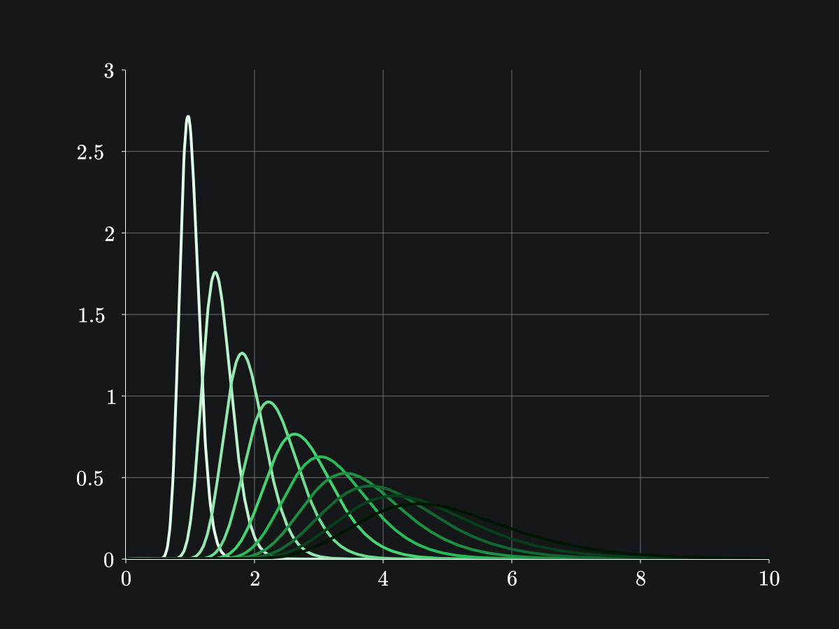
Why do we call this the Log Normal Market Maker?
We call it this because if we look at the liquidity distribution of the pool, we see that it is log normal i.e., normally distributed in the log space:
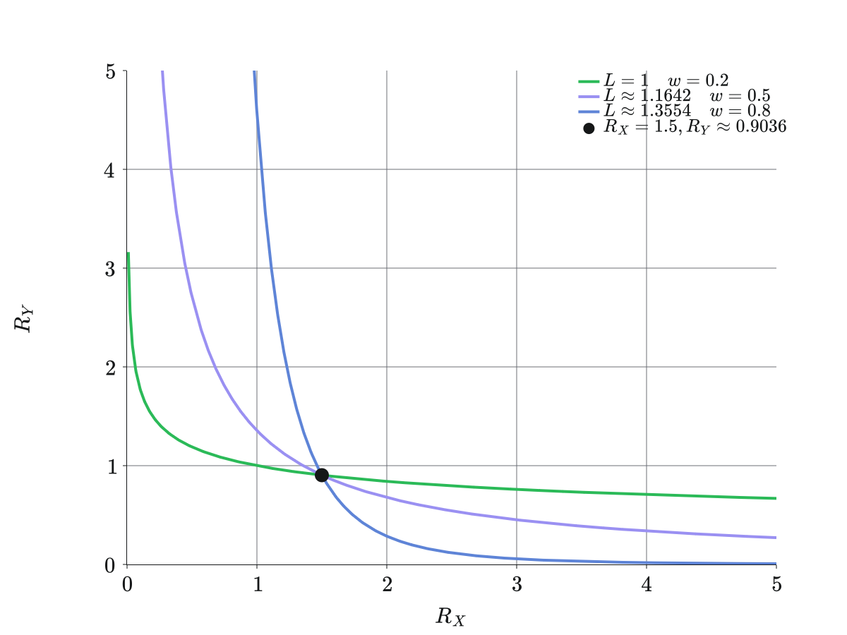
We can see how the trading function behaves as parameters change while reserves remain constant below.
In essence, when parameters change, the resulting curve may not pass through our current reserves, but we are free to rescale the curve using as a scale parameter.
It is necessarily the case that the curve will pass through the reserves for some value of .
The proof is in the picture by taking advantage of the scale invariance of the curve!
Covered Call
Let's consider the DFMM counterpart of the LNMM that adapts the parameters over time. Suppose that we let where is the time to expiry of the pool. Then the DFMM invariant is:
Now, how does, or should, change over time?
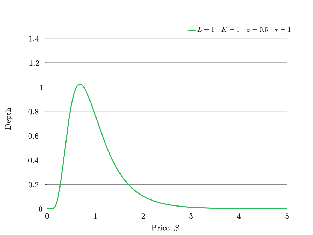
First, let's plot the value of a position with respect to price with liquidity at time :
Note that if then the value of the Black-Scholes Covered Call strategy.
In order for to be constant while decreases, we actually have to effectively increase the reserves and . This is only possible if we apply a fee upon the instruction. Suppose that a user wishes to call with a new state , we can define that if we have that
if the user was swapping in token . This is what we specified in Equation (2) for the instruction. Also, note that I now parameterized using and instead of and for convenience due to the explicit dependence on time in this mechanism.
From this, we can define the trading rule for a valid of the Replicating Portfolio for the Covered Call strategy:
- Update the parameter for the new time , hold reserves constant, and solve to get a new liquidity such that .
- Assert that for satisfies Given (1) and (2), we can see that achieves the payoff of at least the Black-Scholes Covered Call strategy. Keep in mind this comes from Equation (4) above and depends on the fee and trade size.
This extra need to accrue liquidity over time as it is diminished by approaching is equivalent to the positive theta of the Covered Call strategy. Supposing that and no allocations or deallocations were made, then this contributes extra value to the pool that can be thought of as akin to earning a portion of the options premium on the Covered Call over time.
Remark. It is likely not worth enforcing this strict trading rule above as it can lead to the pool being driven into a "dead" state. If it took too long for swaps to occur on the pool, then the pool is effectively behind in its liquidity accrual and thus you require a larger and larger fee revenue on a single swap to get past this gap the longer you wait. Instead, it's best to just ignore this condition and let the pool accrue liquidity as it can.
Liquidity Tracker Strategy
For a second example using LNMM, we can consider a strategy that tracks the liquidity distribution of the pool over time to the emergent token behavior. Current price is intrinsic to the LNMM (and so it falls into block state) and from this we can build a DFMM model that moves and scales the liquidity distribution of the LNMM to track the current price and volatility of the pool. Further, this strategy could employ a dynamic fee parameter to track the volatility of the pool, so we include this explicitly now in .
Take the LNMM with constant and take and to be initially chosen parameters for the pool. Then, we can define the state of the DFMM via . We assert additional conditions on :
- for all (including ).
- where will have volatility in the same units of time as which is the block timestamp at step . This must be picked for by hand. Further, could be averaged out over a history of price changes if desired.
- so that the fee increases for larger price impact trades and the rate of increase is based on a choice of . See exponential distribution.
Remark. This choice of fee parameter was chosen somewhat arbitrarily, but it has the effect of disuading swaps from occuring in periods of high volatility and compensating LPs more for the risk of high volatility. Perhaps it is somewhat like a soft circuit breaker.
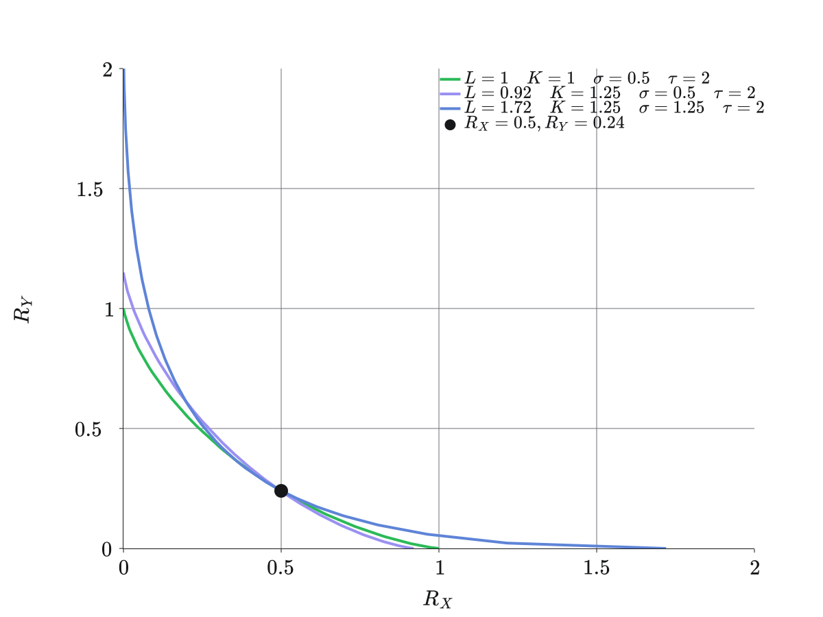
We can see what an example of this would look like.
If we had a market consistently increasing in volatility while the price also increased, our liquidity distribution would adjust like so:
![]() This specific case increased both and as time moved on.
If you wanted to, you could set a parameter range like this for shorter term liquidity management if you expect price to increase, but assume there is random motion in the market (i.e., this matches a drift-diffusion model).
This specific case increased both and as time moved on.
If you wanted to, you could set a parameter range like this for shorter term liquidity management if you expect price to increase, but assume there is random motion in the market (i.e., this matches a drift-diffusion model).
Tokenization
I mentioned previously that this DFMM framework allows for the tokenization of liquidity positions in a pool and we materialized this a bit in the instruction (see Equation (3)). With our framework, DFMM Liquidity Provider Tokens (LPTs) are fungible and can be traded on secondary markets, including placed into other DFMMs, or lent out as collateral, or used as a margin balance. When calling , the user must specify the amount of liquidity they wish to add or remove from the pool as the pool need to handle the reserves and pass the state transition. As worked out before, the amount of reserves added or removed will scale accordingly.
An LP, Alice, will maintain a balance of shares (credited to them on allocation) that represent their claim on the pool's liquidity . The pool itself also tracks an for how many shares (or LPTs) have been created for the pool. Therefore if changes there must be a change in the redemption rate that is used to convert the pools share balance to in order to properly credit the LP such as Alice with the correct amount of underlying tokens upon deallocation.
The process
Upon pool initialization, we can make the assumption that the initial liquidity is the same as the initial share balance of the pool and therefore the initial liquidity redemption rate is . If Alice is the LP who allocated this is given back
LPTs.
- Parameter change: If the parameters of the pool change, then we note that must change as well. Let's assume that the parameter change occurs in the first step, we have and therefore the redemption rate . This means that . Of course, Alice can use her LPTs to make claim on the whole pool, i.e., the new liquidity .
- Swap: If a swap instruction occurs, then if a fee is applied on the swap, then will change again. Assume that this happens at the first step, then we again just have and .
The two cases above resolve to the same problem in tracking change of liquidity that isn't due to an allocation. This is done by keeping an redemption rate between LPTs and pool liquidity .
- Liquidity (de)allocation: In the case that liquidity is allocated at step to , we will know that is the redemption rate. Suppose a new user, Bob, creates a instruction with a , then there is a credit/debit of LPTs to the user's account. The total share balance of the pool is .
Tokenization of DFMM positions provides a new way to compose DeFi tools together and create new products. This design space is quite open and I am excited to see what people come up with.
Wrapping up
This post was meant to be a formal overview of DFMMs and I hope that it has been helpful. If you would like to see implementation details of DFMMs, please see the DFMM-based contracts in the Excalibur repository. Throughout the repo, you can find more details on these two examples as well a Arbiter simulations that are being completed. We plan to rigorously test our implementations and once we are confident in their safety, we will have them deployed. Stay tuned to see some specific instruments we build using DFMMs as primitives. Please get in touch by joining our Discord server if you have any questions or would like to build on top of the DFMM framework.